Archiv des Autors: aud

Save and load

Save and load a R object can be very useful. A common way to store your results in R is to create a txt, csv or xls file. The advantage is that you can open the tables with many programs on your computer. But as soon as you want to do something with it in R it becomes complicated. You need to import the csv file back into R. You need to define header, how the data is separated. And you can never be sure if a factor is still a factor or a date is still a date. Usually, there are some complications that need to be fixed.

An easier solution is to use the function “save” to store your R object. The advantage here is that all the properties of the object are retained. For example a data frame will be a data frame again, a list will be opened as a list.

Let’s create a data set.

# create a data set
petal.length <- rnorm(100, mean = 2.5, sd = 1)
petal.width <- rnorm(100, mean = 1.75, sd = 1)
species <- rep(letters[1:10], each = 10)
floral.traits <- data.frame(species, petal.length, petal.width)

# here we have specis as a factor and two numeric variables
str(floral.traits)
## 'data.frame':    100 obs. of  3 variables:
##  $ species     : Factor w/ 10 levels "a","b","c","d",..: 1 1 1 1 1 1 1 1 1 1 ...
##  $ petal.length: num  2.4 3.08 3.5 2.75 2.92 ...
##  $ petal.width : num  1.525 2.138 2.397 2.148 0.838 ...

Now let us do somthing with this data, for example calculate the mean petal length and petal width for each species.

# calculate mean petal length and withd for each species
mean.pl <- tapply(floral.traits$petal.length, floral.traits$species, mean)
mean.pw <- tapply(floral.traits$petal.width, floral.traits$species, mean)
# transpose the data to make the table easier to handle and combine the means to one data set.
means <- data.frame(t(rbind(mean.pl, mean.pw)))
means$species <- factor(rownames(means)) # add speceis column

We have calculated the mean petal length and width for each species. And now we want to store this result. Maybe we want to use this result later to plot or calculate something. But let’s save it for now with the function “save”.
The first argument is the name of the object you want to save or a list of objects. File is the name of the file with RData at the end. There are more options, but you will mostly use the two first arguments.

# save the R object
save(means, file = "MeanPetalLengthAndWidth.RData")
# let's remove the data set to make sure this is working.
rm(means)

Your R object is now stored in the working directory you are using. We also removed the object from the environment to make sure the object is saved and we can reload it again.

Now we want to load the object back again to our environment to use it further. For this we use the “load” function. The first argument here is the file name. With envir you define where the data should be loaded to. And with verbose you can decide if you want the item name to be printed or not. This can be useful if you have forgotten what it was called.

# load the R object
load("MeanPetalLengthAndWidth.RData", verbose = TRUE)
## Loading objects:
##   means
# check the properties of the object.
str(means)
## 'data.frame':    10 obs. of  3 variables:
##  $ mean.pl: num  2.56 2.34 2.68 2.32 3.23 ...
##  $ mean.pw: num  1.82 1.76 1.75 1.74 2.34 ...
##  $ species: Factor w/ 10 levels "a","b","c","d",..: 1 2 3 4 5 6 7 8 9 10

Now you can check if the object has reapeard in the environment. And then you can . Have fun saving and loading!

# Barplot of petal length
barplot(means$mean.pl, names.arg = means$species, ylab = "Petal length", xlab = "Species")
plot of chunk unnamed-chunk-5

Plant Functional Trait Course in China

The 2016 International Plant Functional Traits Course will offer a hands-on, field-based exploration of plant functional traits, along with experience in the usage of plant traits data in climate-change research and ecosystem ecology. Trait-based ecology offers an important set of methods and new approaches that enables a more powerful approach to predict how climate and biotic interactions shape the diversity of communities and functioning of ecosystems. This course will provide students with the essential background and skills needed for trait-based ecology.

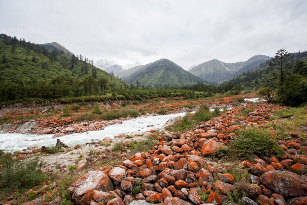
Red stones

Blogging directly from R using RWordPress

My last blog post was published using RMarkdown. It took me a while to intall all the packages needed but the publishing was very easy.In fact, it is 2 lines of code. But let’s start with the hard part getting all the packages installed and running.

The RWordPress package is currently on github (February 2016). It can be installed directly from there, but for that the devtools package is needed. To connect to WordPress we need the XMLRPC package. And you need of course the RWordPress package and the knitr package to make the blog post.

Let’s install the packages.

install.packages("devtools")
library(devtools)

install_github("duncantl/XMLRPC")
install_github("duncantl/RWordPress")
install.packages("knitr")

library(XMLRPC)
library(RWordPress)
library(knitr)

Once your blog post is writen you can check how it looks. For this you press the “Knit HTML” button on top (in R Studio). If everything looks fine, you are ready to publish. With options you define your username, password and url with “xmlrcp.php” at the end.

In “knit2wp” you define the filename of the Rmd document and the title of the blog post. You can publish directly, but by setting publish = FALSE you can make a draft and publish it later. With action you can create a new or edit an existing post.

options(WordPressLogin = c(user = 'Password'), WordPressURL = 'https://audhalbritter.com/xmlrpc.php')
knit2wp('RWordPress.Rmd', title = 'Blogging directly from R using RWordPress', publish = FALSE) 

You can find more information here and here:
http://yihui.name/knitr/demo/wordpress/
http://3.14a.ch/archives/2015/03/08/how-to-publish-with-r-markdown-in-wordpress/

Have fun bloggin!

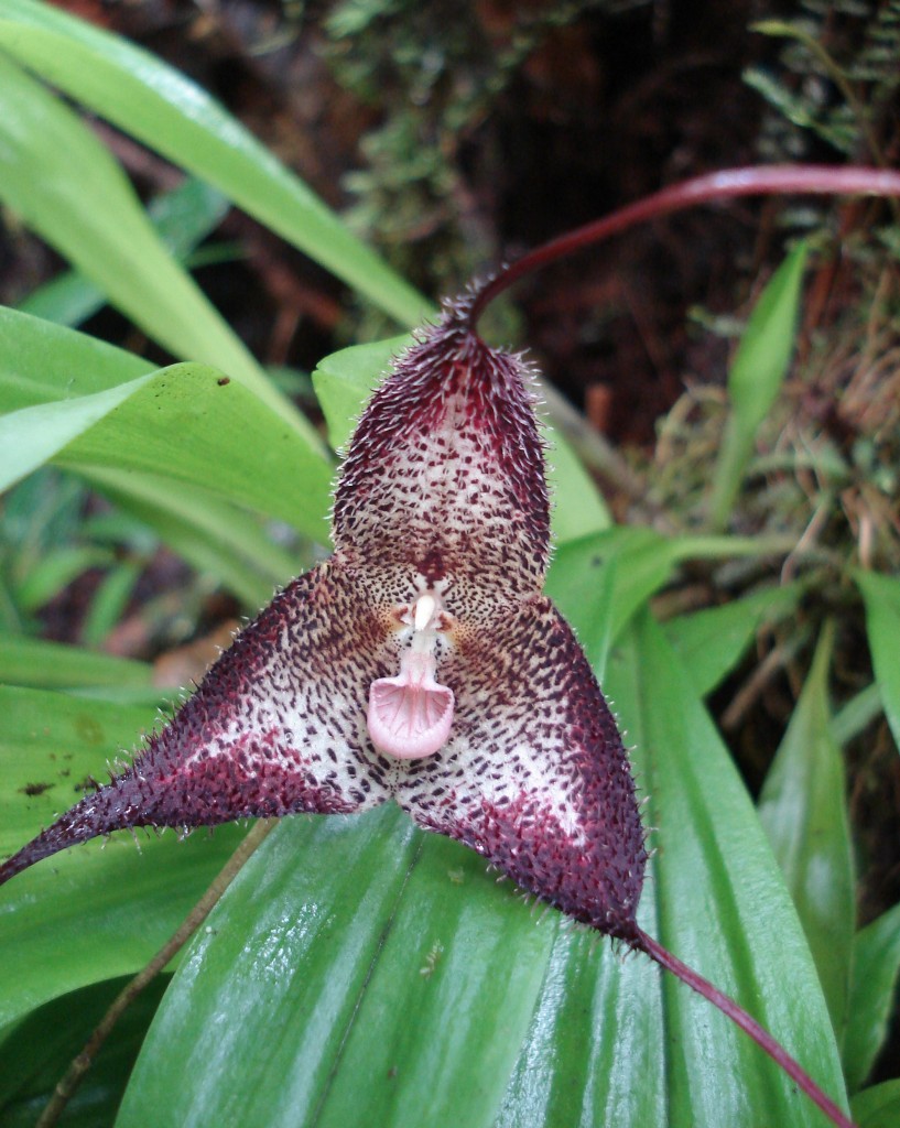
New article on mushroom-mimickring Dracula orchids and 3D printed flowers

Tobias Policha and collegues published an interestig article how they used 3D printed flowers to disentangle visual and olfactory signals in an orichid. You can get to the article here. The picture shows a Dracula lafleurii.

Dracula lafleuriicropped

Flowers use olfactory and visual signals to communicate with pollinators. Disentangling the relative contributions and potential synergies between signals remains a challenge. Under- standing the perceptual biases exploited by floral mimicry illuminates the evolution of these signals. Here, we disentangle the olfactory and visual components of Dracula lafleurii, which mimics mushrooms in size, shape, color and scent, and is pollinated by mushroom-associated flies.

 To decouple signals, we used three-dimensional printing to produce realistic artificial flower molds that were color matched and cast using scent-free surgical silicone, to which we could add scent. We used GC-MS to measure scents in co-occurring mushrooms, and related orchids, and used these scents in field experiments.

 By combining silicone flower parts with real floral organs, we created chimeras that identi- fied the mushroom-like labellum as a source of volatile attraction. In addition, we showed remarkable overlap in the volatile chemistry between D. lafleurii and co-occurring mush- rooms.

 The characters defining the genus Dracula – a mushroom-like, ‘gilled’ labellum and a showy, patterned calyx – enhance pollinator attraction by exploiting the visual and chemosen- sory perceptual biases of drosophilid flies. Our techniques for the manipulation of complex traits in a nonmodel system not conducive to gene silencing or selective breeding are useful for other systems.

Picture from: http://cascade.uoregon.edu/fall2010/natural-sciences/natures-masters-of-disguise/

Using the by function in R

Recently, I have discovered the by function in R. With “by” you can apply any function to a data frame split by a factor. Yes, this sounds difficult, but I will show you how powerful this function is with an example.

Let’s say we have measured petal width and length of 10 individual flowers for 3 different plant species. The data frame has 3 columns (species, petal width and petal length) and 30 rows (3 species x 10 individuals). Here is the code to make this data frame:

# Create a data frame with petal length and petal width for 3 species
dat <- data.frame(species=c(rep(c(1,2,3), each=5)), petal.length=c(rnorm(5, 4.5, 1), rnorm(5, 4.5, 1), rnorm(5, 5.5, 1)), petal.width=c(rnorm(5, 2.5, 1), rnorm(5, 2.5, 1), rnorm(5, 4, 1)))

dat$species <- factor(dat$species) # make species a factor

dat
##    species petal.length petal.width
## 1        1     4.036443   4.2636530
## 2        1     4.805463   2.9856014
## 3        1     4.416011   2.2342611
## 4        1     4.910363   2.6516114
## 5        1     4.683678   3.8766098
## 6        2     6.278742   2.3196057
## 7        2     4.537683   0.9323249
## 8        2     5.676220   2.2392741
## 9        2     3.941464   3.4618104
## 10       2     3.554382   3.3538955
## 11       3     4.834811   4.4187967
## 12       3     5.952030   4.3399565
## 13       3     6.026856   4.5964251
## 14       3     5.269738   5.8714180
## 15       3     6.897427   4.6028704

We can use the by function to calculate the mean petal length for each of the three species.

The first argument is which data frame you want to use. Next you specify by which factor you want split your data frame. And finally you say which function you want to use. In our case this is the mean.

by(dat, dat$species, function(x){
  # caculate the mean petal length for each species
  mean.pl <- mean(x$petal.length)
})
## dat$species: 1
## [1] 4.570392
## -------------------------------------------------------- 
## dat$species: 2
## [1] 4.797698
## -------------------------------------------------------- 
## dat$species: 3
## [1] 5.796172

There are easier ways to calculate the mean of 3 species. But if you have understood the principle of the function, you can use it to do more complicated calculations. Here is another example, to draw a scatter plot for the petal width and petal length and drawing the regression line for each of the three species.

par(mfrow=c(1,3))
by(dat, dat$species, function(x){
    # caculate the mean petal length for each species
  mean.pl <- mean(x$petal.length)

  # draw a plot for each speceis
  plot(x$petal.width, x$petal.length, xlab="petal width", ylab="petal length", ylim=c(2,8))
  abline(lm(petal.length ~ petal.width, x), lty=2)
})

plot of chunk unnamed-chunk-4

You might have noticed that the output looks a bit strange. This is because the output of the by function is stored in a list. List’s are complicated but also extremely powerful. For example, a data frame needs to have the same number of entries in each row or column. A list can have entries that different in length, which can be very useful at times.

But here is a little trick to get your output back into a data frame using sapply.

sp.means <- by(dat, dat$species, function(x){
# caculate the mean petal length and petal width for each species
  means <- colMeans(x[,2:3])
})

# use sapply to put the data back to a matrix
sp.means2 <- t(sapply(sp.means, I))
# make a data frame
new.df <- as.data.frame(sp.means2)
new.df
##   petal.length petal.width
## 1     4.570392    3.202347
## 2     4.797698    2.461382
## 3     5.796172    4.765893

New article from our lab in GCE on population dynamics in grasslands

From facilitation to competition: temperature-driven shift in dominant plant interactions affects population dynamics in semi-natural grasslands

Siri L. Olsen, Joachim P. Töpper, Olav Skarpaas, Vigdis Vandvik and Kari Klanderud

Biotic interactions are often ignored in assessments of climate change impacts. However, climate-related changes in species interactions, often mediated through increased dominance of certain species or functional groups, may have important implications for how species respond to climate warming and altered precipitation patterns. We examined how a dominant plant functional group affected the population dynamics of four co-occurring forb species by experimentally removing graminoids in semi-natural grasslands. Specifically, we explored how the interaction between dominants and subordinates varied with climate by replicating the removal experiment across a climate grid consisting of twelve field sites spanning broad-scale temperature and precipitation gradients in southern Norway. Biotic interactions affected population growth rates of all study species, and the net outcome of interactions between dominants and subordinates switched from facilitation to competition with increasing temperature along the temperature gradient. The impacts of competitive interactions on subordinates in the warmer sites could primarily be attributed to reduced plant survival. Whereas the response to dominant removal varied with temperature, there was no overall effect of precipitation on the balance between competition and facilitation. Our findings suggest that global warming may increase the relative importance of competitive interactions in semi-natural grasslands across a wide range of precipitation levels, thereby favouring highly competitive dominant species over subordinate species. As a result, semi-natural grasslands may become increasingly dependent on disturbance (i.e. traditional management such as grazing and mowing) to maintain viable populations of subordinate species and thereby biodiversity under future climates. Our study highlights the importance of population-level studies replicated under different climatic conditions for understanding the underlying mechanisms of climate change impacts on plants.

How to prepare a manuscript for publication?

If you are a scientist, you want to publish your work at some point. Other scientists in your field should read and learn from your work. And in science a publication is usually a paper in a journal. Publishing a paper can be hard work if you do it for the first time (also later), but you’ll learn and get better at it. The first step is to prepare a manuscript that you send to a journal. Here are some of my experiences, how to do it.

I am an ecologist and some things might only apply to this field, but I think most journals have a similar style and these ideas can be used everywhere.

Each journal will provide author guidelines. It is very important to read these very carefully before starting anything. The journals specify what type of articles they are interested in. Think carefully if your study fits into the journal. A good idea is to look at a recent issue to see what kind of articles there are. Some journals ask for an abstract before telling you if they want you to send in the full manuscript. Another important point to check is if you are ok with their conditions? For example, some journals want you to provide your data, or in some journals you have to pay for colour figures. Make sure you are aware of their requirements.

Content and structure

  • Language: most articles have to be written in English. If you are not a native English speaker it is a good idea to let a native speaker read your text or somebody with lot’s of experience.
  • Title: add a short and catchy title. It’s the first thing your reader will see!
  • Whatever you do, be consistent throughout the manuscript: use the same expressions for things and write in the same style.
  • The key words should be words not used in the title but important terms in the manuscript
  • Usually research articles follow this structure: title page, abstract, introduction, method and materials, results, discussion, acknowledgements, references, tables, figure captions.
  • What information is needed on the title page?
    • Title
    • Author names and their affiliation, email address
    • Running title: is an abbreviated title, which is usually printed at the top of the text pages and allows the reader to determine which paper they are looking at.
    • Corresponding author: is usually the author that is responsible for the correspondence throughout the publication process.

Formatting style

  • Use a recent paper as a template. Not to copy but as guidance.
  • Add line numbering: it’s easier for anybody reading your text to refer to a specific position in your text.
  • Double spacing makes the text more readable.
  • Do not justify the right margin. It is maybe not as aesthetically pleasing, but far more readable.
  • Add page numbers! Have you ever printed a 30-page text and then mixed the pages?
  • Keep to the word count or page allowance. If you don’t, it is very easy for the editor to reject your manuscript.
  • Check the requirements for figures and tables: quality of figures, where and how to place the legend, are coloured figures allowed or do you need to pay for it and how should you refer to them (Fig. 1a or Figure 1A). How do you submit figures and tables? Some journals want them in the text (e.g. one table per page), some want you to upload the figures separately.
  • How does the supplementary material need to be presented? In a separate file? And how should you refer to the supplement material (see Appendix Fig. S1)?
  • What format of your manuscript is allowed? Word, LaTex, PDF,…
  • Check your reference list very carefully! Number allowance, format, order. It is very easy to make mistakes here and not all programs provide correct references. Are the species names in italics? Usually there should not be Capital Letters in the Title unless it is a Location or a Name.

By following these instructions, it is not guaranteed that your paper gets accepted. But if you keep to “the code” the editor is more willing to have a real look at the content of your manuscript and not send it back right away.

Good luck preparing your first manuscript and let me know about your experiences.

Create a map in R

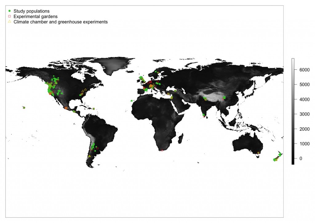
I belive that every ecological publication of a study needs a map. It does not necessarily need to be in the paper but at least in the appendix. I admit, I like maps and could look at maps for infinity, but maps also illustrate where a study was done, the scale of the study and where populations were collected, the range of the study species or locations of the study can be visualized.

Making maps is very easy with R. With a few lines of code you can produce a map of any region in the world and then plot points on the map.

Here, I produced a world map using the worldclim elevation data as background and plotted populations and study sites on the map. I used raster package, which is a powerful tool to process spatial data.

This is the R code I used for the map:

install.packages(„raster“)
library(raster)
climate <- getData(‚worldclim‘, var=’alt‘, res=2.5) # download elevation data from worldclim

plot(climate$alt, axes=FALSE, col = grey(0:100/100)) # plot world map
points(dat.pop$long.pop, dat.pop$lat.pop, col=“limegreen“, pch=16, cex=0.7) # plot populations
points(dat.site$longitude_site, dat.site$latitude_site, col=ifelse(dat.site$studysite==“Garden“,“firebrick1″, „gold1″), pch=ifelse(dat.site$studysite==“Garden“,0,2), cex=0.8) # plot sites
legend(„topleft“, c(„Study populations“, „Experimental gardens“, „Climate chamber and greenhouse experiments“), pch=c(16, 0,2), col=c(„limegreen“, „firebrick1“, „gold1″), bty=“n“)

Worldmap


Other powerful packages to draw maps are maps and mapdata. To plot maps there is a simple command „map“. And by adding a country or a list of countries only parts of the world are plotted.

library(maps); library(mapdata)
map(‚worldHires‘) # the world
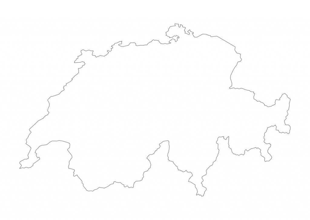
map(‚worldHires‘,’Switzerland‘) # Switzerland
map(‚worldHires‘, c(‚Norway‘, ‚Sweden‘, ‚Finland‘,’Denmark‘, ‚Island‘), xlim=c(-11,50), ylim=c(45,90)) # Scandinavia


Switzerland

Application for a Landrover

This week two collegues and me applied for a landrover for the next field season. The grant is from the Royal Geographic Society: „The award is aimed at those who want to take a journey beyond their limits and boundaries, that offers chalenges for the team.“

To illustrate our motivation and that a good car is an essential part of our field work we created a video about our project.