Summerfield, R. J. 1999. Timing it right: the measurement and prediction of flowering. – Acta Agron. Hung. 47: 203–213.
Sack L, Cornwell WK, Santiago LS, Barbour MM, Choat B, Evans JR, Munns R, Nicotra A. 2010. A unique web resource for physiology, ecology and the environmental sciences: PrometheusWiki. Functional Plant Biology 387: 687-693.
IPBES (2019). Summary for policymakers of the global assessment report on biodiversity and ecosystem services of the Intergovernmental Science-Policy Platform on Biodiversity and Ecosystem Services.
Archiv der Kategorie: Allgemein
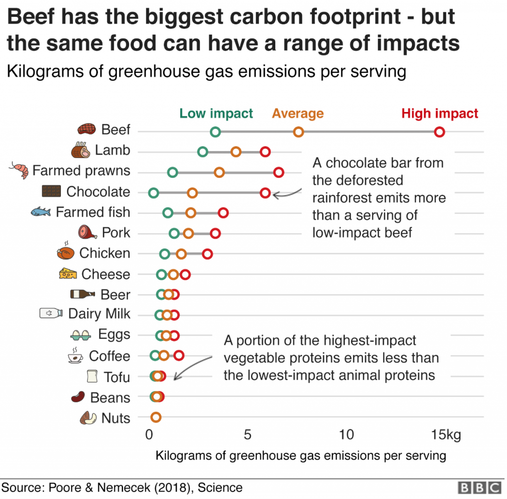
The carbon footprint of your food
A new study from Poore & Nemecek shows the carbon footprint of our diet. BBC’s has made a tool, where you can check the carbon footprint calculator for what you eat. Not surprisingly, reducing meat and diary products reduces your environmental impact most (Poore & Nemecek, Science, 2018).
First field day – THREE-D
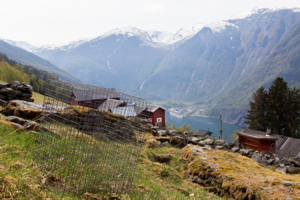
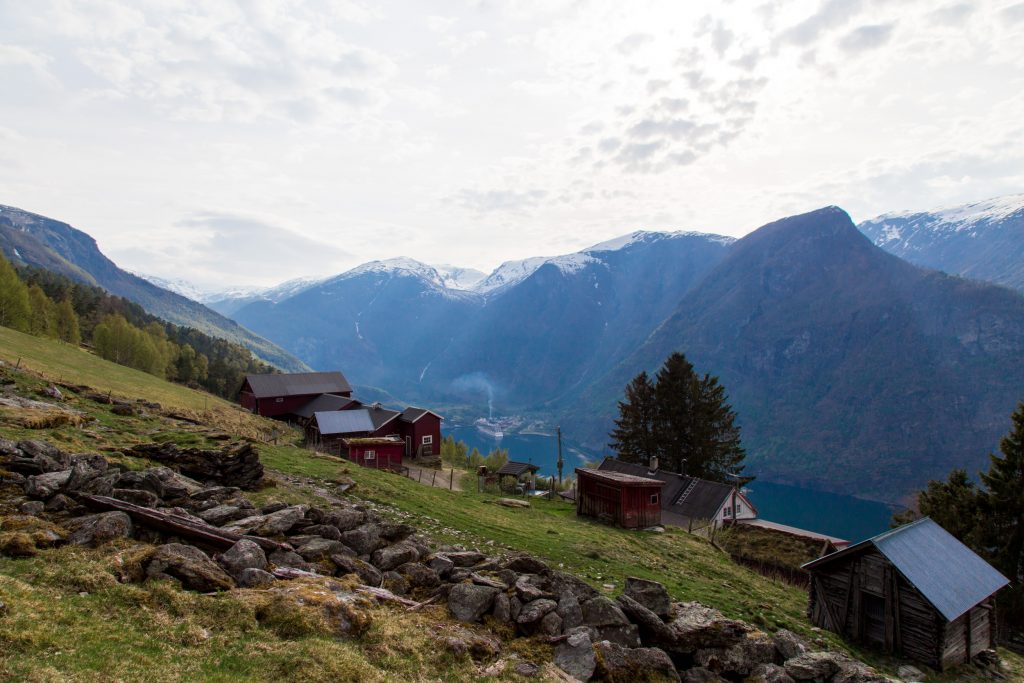
A couple of weeks ago, I went to the field for the first time in the THREE-D project. In this project, we want to disentangle the impact of different global change drivers on biodiversity and the carbon cycle. We need to select new sites and set up the whole experiment this summer in western Norway and eastern Himalaya in China.
This first round was to set up grazing exclosures. We want to get and estimate of the grazing intensity along the elevational gradients, to know how much biomass is removed over the growing season. For this, we put up metal cages, that will exclude large herbivores and this will be compared with control plots without cages. The biomass in these plots will be harvested, dried and weighed. A master student will work on this project in Norway this summer.
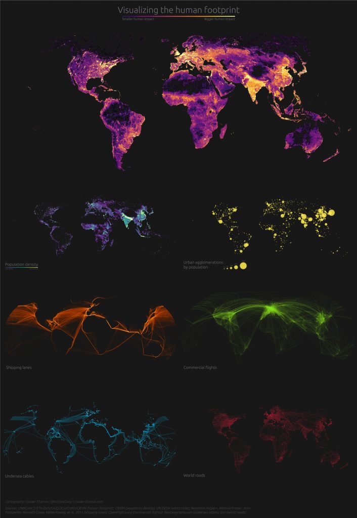
Anthropocene
Seven maps showing the human footprint. Made here.
THREE-D project: new page
There is also a new page about the THREE-D project here.
THREE-D webpage
The Three-D project has a webpage!
Reading list 18. – 24.3.2019
Delgado-Baquerizo et al. 2019. Changes in belowground biodiversity during ecosystem development. PNAS.
Wardle et al. 2004. Ecological Linkages Between Aboveground and Belowground Biota. Science. 304, (5677), 1629-1633.
Adair et al. 2019. Above and belowground community strategies respond to different global change drivers. Scientific Reports. 9: 2540.
Part 2 – From chicken foot to raspberry pi
Learning – how to measure plant functional traits – the hard way (a story in 4, or more, parts)
This is the story of how we organized our TraitTrain courses and what we learnt from our mistakes. With TraitTrain we want to strengthen research and educational collaborations over climate change and ecosystem ecology by organizing courses for students on how to measure plant functional traits and at the same time offer the students a relevant research experience. In the first part I explained how we organized the collection of the leaf traits, the so called trait wheel. Here, I want to talk about the 3rd step in the trait wheel: scanning the leaves.
Leaf area is a common measure of leaf size and is usually very plastic to climatic variation and/or stress. Leaf area is also important because it is used to calculate SLA (specific leaf area). To calculate leaf area, a leaf is scanned (for details see Pérez-Harguindeguy et al. 2013) and the scan is then run through a program such as ImageJ, which calculates the area of the leaf. We use ImageJ via the r package LeafArea.
All of this should be easy, except it wasn’t.
On the course each student had a laptop, which we then connected to the scanners. We usually have 4-5 scanners, because this is a time demanding job. On the TraitTrain courses, we have students from all over the world and they come with all sorts of laptops (brands, operating systems and settings). The instructions said to scan the leaves with specific settings (e.g. 300 dpi). For some reason, the scans from people with different settings on their computers (A4, letter,…) resulted in different leaf areas. We are still not sure how this happened, because when you set the resolution, the size of a scan should not make a difference.
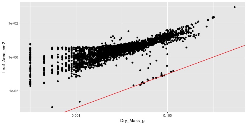
The second problem was that many pictures had black edges around them (see picture 1), which was added to the leaf area. We did not understand this until we plotted leaf area against dry mass, which should be a more or less linear relationship. Instead the plot looked like a chicken foot (this expression might also have been inspired by all the chicken feet that were swimming around in our hotpots). It tooks us a while to figure this out and we had to look at each individual scan to make identify several of these problems.

How did we solve these issues for the next courses. First of all we wanted to make the scanning a standardized process and not dependent on the settings of peoples laptops. We bought a couple of raspberry pi’s, which operated the scanners. We used the laptops as screens and keyboards to operate the scanner and pi’s.
Second, we implemented a couple of checks. The pi automatically checked if the scanning settings were correct (resolution, size, colour depth, file type), if the person scanning the leaf had typed in the correct LeafID and if the scan was saved in the right place. If you are interested in how we set up the pi and scanner, all the scripts we used is available on github.
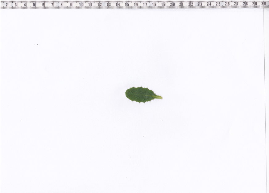
We also realized that for checking the quality of the data and finding errors, we need a size reference on each scan. For this we added a ruler to each scanner (ruler glued to each scanner; see picture 2), which allowed us to directly check if the leaf area was calculated approximately right. This turned out to be very useful. One problem that occurs is of course you do not want to have the ruler on the scan when you calculate leaf area. The LeafArea package allows to cut a certain amounts of pixels on each side of the scan. This is very useful and also solves the problem with the black lines. The problem was now that we could only cut the same number of pixels on each side. But what we wanted was to cut more on the side where the ruler was added and less on all the other sides of the scan. For this we customize the run.ij function in the LeafArea package. If you want to use our customized run.ij function, run this code first in r devtools::install_github(„richardjtelford/LeafArea“). Then the run.ij function has an argument “trim.pixel2”, which allows to cut more pixels on the right side of the scan.
Visual inspection of each scan turned out to be essential even by optimizing the scanning process. It is important to check the right number of pixels are cropped before calculating the leaf area, you can check that the full leaf is scanned and you can detect folded leaves. By checking each individual scan, we also found that some of the scans were really dirty. This happens, when working with plant material that comes from the field. And now, we tell the students to check and clean the scanner often. And finally, grasses can be difficult, because they tend not to lie flat on the scanner. They curl. Here, the answer was to use transparent tape to glue the leaves onto the scanner.
Part 1: The invention of the trait wheel
Learning – how to measure plant functional traits – the hard way (a story in 4, or more, parts)
TraitTrain is a group of plant ecologists from the Universities of Bergen in Norway and Arizona (USA). We want to strengthen research and educational collaborations over climate change and ecosystem ecology. We are organizing courses for students on how to measure plant functional traits and at the same time offer the students a relevant research experience, i.e. by being part of a real research project and collecting real data. Being part of a projects is more motivating for students than collecting “dummy data”. This is a challenging goal and does not always work out. Here, I want to explain how we organize these courses and what we learned from our mistakes. In a couple of next blog posts, I want to discuss how to ensure data quality, technical problems and solutions, next steps and unresolved problems.
On our team, we have an extremely successful person getting research grants (basically our boss), and she is also obsessed with education and collecting all sorts of data. She secured the money to organize the trait courses. Also, we have many colleagues who were willing to travel to cool places (China, Peru, Svalbard) and teach functional trait and climate change ecology. Finally, we have hospitable Chinese, Peruvian, Icelandic and Norwegian collaborators with field sites at the edge of the Tibetan Plateau (Sichuan, China), in the Andes (Peru) and Svalbard (Longyearbyen, “Norway”) willing to let a hoard of students lose on their field sites and experiments. Not sure, if I would…
What is the big deal with organizing a course with a couple of students? There is nothing special about that, and hundreds of people have done this before. The special thing with our courses was, that we did not only want to teach about traits and climate change ecology; we also wanted to collect a publishable data set. And this is where it gets tricky. The good thing about all the students is that a huge amount of data can be collected in a short time. The downside, it can go horribly wrong and instructions need to be given very explicitly to collect the data in a standardized way. The problems can be passed along from one student to the next and errors accumulate.
The basic principle of measuring leaf traits is to go to the field, collect plants, bring them back to the lab where traits are measured (see video below): plant height, wet mass, leaf area, thickness. Then the leaves are dried and weighed again for dry mass. From the dry leaves, chemical traits for example carbon and nitrogen content can be measured. To get a decent data sets, you need trait measurements from different species, leaves and locations, and you will end up measuring hundreds of leaves. A tedious task! Our first strategy was the trait wheel, which has turned out to be very useful. The trait wheel is organizing the different trait measurements in separate stations and each leaf has to go through each station in a fixed order. And each station is manned by several students.
We followed the trait handbook by Pérez-Harguindeguy et al. (2013) and I am not repeating the basics of plant collections and trait measurements. Rather, I will highlight useful tips that we learnt from our mistakes.
The first step (not yet a station), is to collect the plants or leaves in the field. Where and how to collect leaves is important, but I will not go into detail here. This step depends on your research question and there are some useful guidelines on sampling strategies in the trait handbook. It is useful to measure plant height already in the field (unlike in the video!). Measuring plant height in the lab works well for “stiff” plants. But for plants that bend easily (e.g. grasses) it is hard to get the plant height right after the plant has been picked from the ground. We also found it useful to use a separate plastic bag for each plant. Yes, we used a lot of bags (we cleaned and reused the bags), but all information (date, site, species, height, collector, etc.) can be written directly on each bag and fewer plants get lost and information lost.
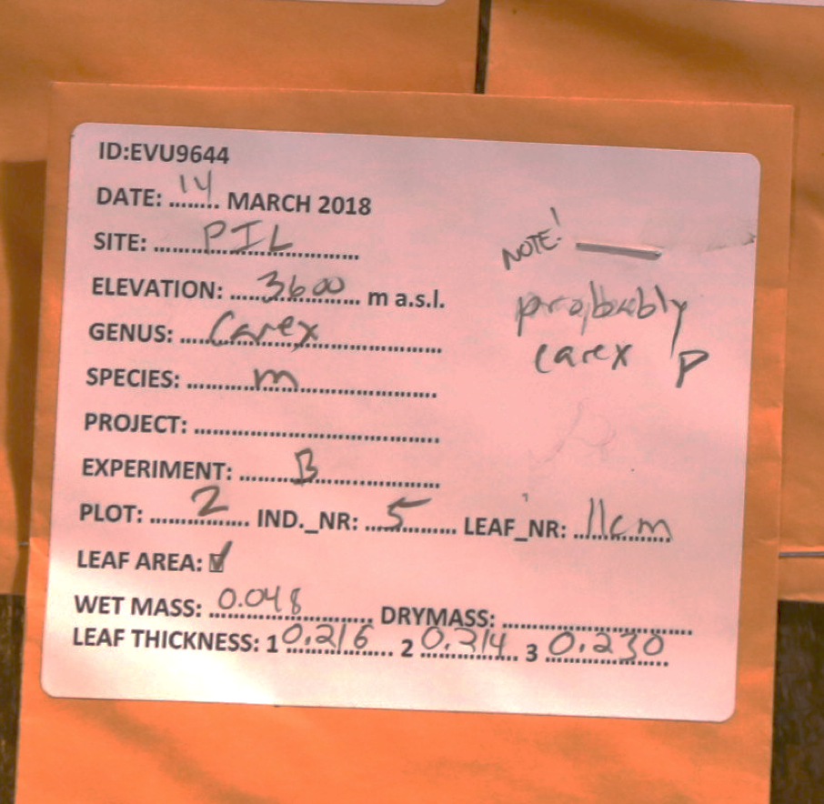
When a leaf arrives in the lab, it goes to station nr. 1 the preparation and labelling. Here, the plants are identified (if this has not already happened in the field), the leaves selected, put into an envelope and labelled. This is a crucial step and people with species identification skills are needed. Leaves that are labelled wrong or go in the wrong bag are difficult to fix later. Another point is to make sure, that each envelope is labelled with the necessary information. We learnt that even if you have to remember to note down the same 5 things, it is hard, and students (and professors) forget to write crucial information on the envelopes. To help the students to remember all information, we preprinted labels with blanks and boxes (see Photo). We used sticky labels that could be easily glued to each envelope. At each station, the data is entered or boxes are ticked. This reduced a large amount of errors.
The preparation and labelling station is also when you decide how much plant material goes into one envelope. Usually one leaf is enough, but if the leaves are very small you might want to go for a bulk sample (several leaves from one individual). The amount of plant material is important for the chemical analysis where a certain amount of plant material is needed. Plan this step ahead and make sure you know how much plant material you need (dry weight!).
The next station is nr. 2 wet mass. This is not a particular difficult task. The important thing here is to have a balance that measures your leaves with sufficient accuracy. This is again important for small leaves, for example in arctic and alpine habitats.
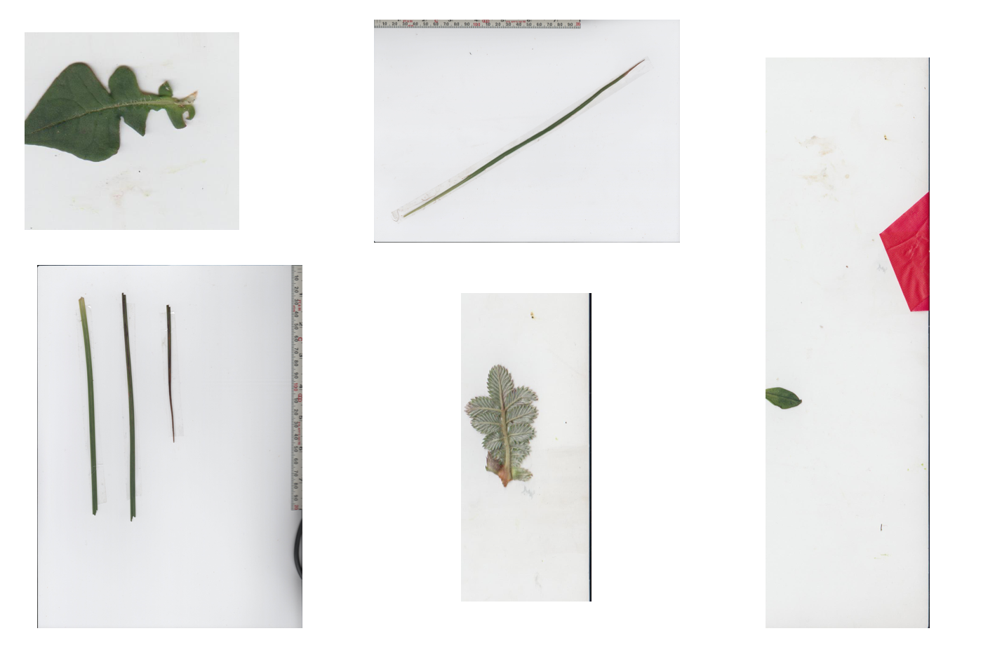
Station nr. 3 is scanning leaf area. A leaf is scanned using a normal scanner, and the area calculate using a software like ImageJ. It is important to scan the leaves upside down, scan the whole leaf (large leaves can be cut), keep leaves flat and not rolled (tape can be used to keep leaves flat) and not scan other things (e.g. cables, tissues; see photo). Keep the scanner clean at all times, because large dust and dirt particles will be counted as part of the leaf. And finally, have a ruler (to measure size) on each scan as reference object. There will be a separate blog post on the scanning process.
Station nr. 4 is measuring leaf thickness. A digital caliper should be used and this step will take a lot of time. It is good to have 3-4 people working on this at all times.
Next the leaves go into the drying oven and are weighed again (dry mass; same as station nr. 2). This step can be done later and this was usually done after the course.
Station nr. 5 is data entering. It is useful to enter the data right away and more importantly check the data. If data is missing or values are wrong (e.g. too high or small), a leaf might be reweight or measured if it has not been dried yet. Prepare the data entering sheet beforehand. There will also be a separate blog post on data quality checking.
Here are some last words on organizing the trait wheel. The students should work on one station for a while but make sure to rotate, so that everybody works at each station. It is important that the boss/teacher/organizer has the overview of the trait wheel! Who has worked on which station, who goes to the field, when do the students rotate.
The leaves should be kept moist until drying, because they should be as fresh as possible. We had a box with moist paper in a plastic bag at each station, where the envelopes were kept moist. Further, it is not advisable to process too many leaves at the same time. It is important that each station is manned at all times, and slow stations need more people. Leaves should not be lying around between stations for too long. Towards the end of the day, the first stations have to stop to make sure that all leaves go through the trait wheel on the same day. Leaves can be kept moist overnight, but it is better to finish them.
Our courses are rather intensive and repetitive for the students. We try to make the course more diverse by giving lectures, have student presentations and give them a day off (very important!). One crucial thing is that the students understand each step of the trait wheel (i.e. what trait is measured and why). Ideally, the students do not see this data collection as a boring and repetitive task, but they think for themselves and report errors and fix them. For this, the students need to be motivated, interested and understand the importance of functional leaf traits, data quality and large data sets.
Readling list 28.1 – 3.2.2019

Cooper et al. 2018. Genotypic variation in phenological plasticity: Reciprocal common gardens reveal adaptive responses to warmer springs but not to fall frost. Glob Change Biol, 25:187–200.
Forest and Thomson. 2010. Consequences of variation in flowering time within and among indiviuals of Mertensia fusiformis (Boraginaceae), an early spring wildflower. American Journal of Botany 97(1): 38–48.
Diez et al. 2012. Forecasting phenology: from species variability to community. Ecology Letters, 15: 545–553
Khorsand Rosa et al. 2015. Plant phenological responses to a long-term experimental extension of growing season and soil warming in the tussock tundra of Alaska patterns. Global Change Biology,21, 4520–4532.
Zhang et al. 2017. New insights on plant phenological response to temperature revealed from long‐term widespread observations in China. GCB.
Arnold et al. 2018. How to analyse plant phenotypic plasticity in response to a changing climate. New Phytologist.