Archiv der Kategorie: Allgemein

ggplot with colour, shape and colour depending fill

Everything is possible with ggplot in R. I realized that again today when plotting some climate data with different colour, shapes and fill. Color showed different precipitation levels, shape showed different temperature levels and I wanted filled symbols for the short term data and filled symbols for the long term data set. The complication was that the filled symbol depended as well on the precipitation level.

My solution was to manually fit different colours for fill, but this messed up the legend. So here comes trick number 2 to manually change the legend.

Let’s have a look at the plots and create a data set. There are 2 climate variables: temperature and precipitation. A factor for temperature and precipitaion with each 2 levels to define color and shape. And the source of the data (short or long term data).

# create a data set
Data <- data_frame(Temperature = c(8.77, 8.67, 7.47, 7.58, 9.1, 8.9, 7.5, 7.7),
                   Precipitation = c(1848, 3029, 1925, 2725, 1900, 3100, 
                                     2000, 2800),
                   Temperature_level = as.factor(c(rep("subalpine", 2), 
                                                   rep("alpine", 2), 
                                                   rep("subalpine", 2), 
                                                   rep("alpine", 2))),
                   Precipitation_level = as.factor(c(rep(c(1,2),4))),
                   Source = c(rep("long term", 4), rep("short term", 4)))

Let’s plot the data using ggplot. We want the filled symbol to be according to the precipitation level. So we use a ifelse statement for fill. If the source is the short term data, then use the precipitation colours, otherwise not. And manually we define the two blue colours and white for the symbols we do not want to have filled.

p <- ggplot(Data, aes(x = Precipitation, y = Temperature, 
                      color = Precipitation_level, 
                      shape = Temperature_level, 
                      fill = factor(ifelse(Source == "short term", 
                                           Precipitation_level, Source)))) +
  scale_color_manual(name = "Precipitation level", 
                     values = c("skyblue1", "steelblue3")) +
  scale_shape_manual(name = "Temperature level", values = c(24, 21)) +
  # manually define the fill colours
  scale_fill_manual(name = "Source", 
                    values = c("skyblue1", "steelblue3", "white")) +
  theme_minimal()
p + geom_point(size = 3)

plot of chunk unnamed-chunk-3

The colours, shape and fill was plotted correctly, but this trick messed up the legend for the data source. The reason is that fill has 3 levels: 2 precipitation levels and one level for the long term data, which we coloured white.

We need another trick to fix this. We will use another factor with 2 levels and then replace the fill legend. First, we add different size for Source. It can be marginally different or have exacly the same value. This seems silly, but it’s useful to change the legend for fill. For changing the legend “guides” is a useful function. First we remove the fill legend. Then we use size which only has 2 levels and use override to draw different shapes for the two levels. And these shapes represent the filled and unfilled symbols.

p + 
  # add size for Source
  geom_point(aes(size = Source)) +
  # defining size with 2 marginally different values
  scale_size_manual(name = "Source", values = c(3, 3.01)) +
  # Remove fill legend and replace the fill legend using the newly created size
  guides(fill = "none", 
         size = guide_legend(override.aes = list(shape = c(1, 16))))

plot of chunk unnamed-chunk-4

So, everything is possible in ggplot. It’s not straight forward code and needed a few tricks to make it work. If you know a quicker way to draw this plot, please let me know!

Thanks, Richard for helping with trick nr. 2!
Landpress project

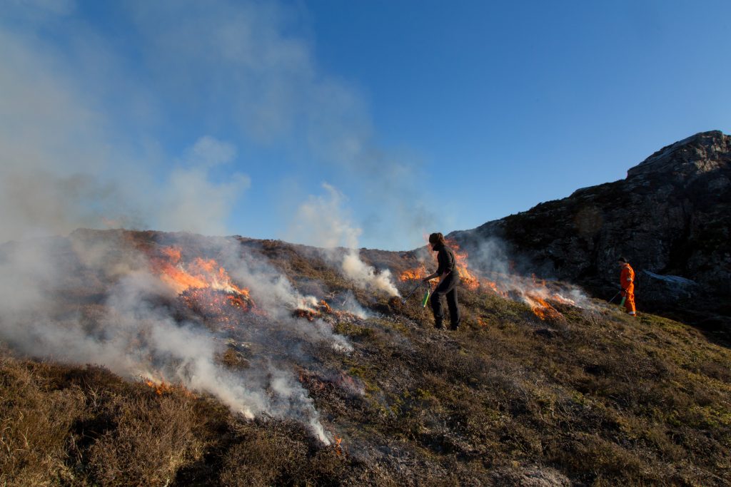
Heathland are costal habitats shaped by humans hundreds of years ago. They were burned to clear the land for their animals. Burning the heathland was continued to improves the fodder quality and prevent shrubs and trees to grow in the heathland.

In 2014 an intensive drought led to heather death along the coast of Norway. Landpress tests whether heather burning is an effective measure to prevent drought damage and restore damaged moorland.

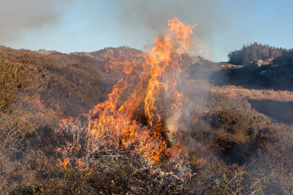
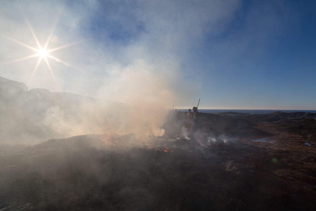
Last week, one of the sites, close to Bergen was burned.

RMarkdown presentation – title page picture

Creating presentations with RMarkdown in R is a useful alternative to using Power Point. It is very useful for code loaded presentations. But many people produce the results (figures) they present in R. And whenever something is changed in the data or code each figure has to be remade, save again and exchanged in the presentation. RMarkdown will do all that automatically.

But let’s start at the first page. Most presentations (that I have seen) have a picture on the title page, because pictures say more than words. So how do you put a picture on your RMarkdown presentation?

It took me a while to figure out, but it’s quiet easy. I assume you know how to get started with your presentation. Otherwise check out this link.

The first thing you need to fix are the first couple of lines in your RMarkdown file. After output you write: ioslides_presentation: css: styles.css

Bildschirmfoto 2016-08-25 um 21.10.17

Make sure the spacing is right! This will tell your RMardown to look for a css file.

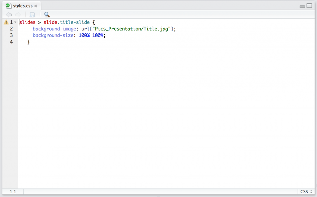
The next step is to create a css file. Where you then can define all sorts of things, for example to put a picture on your title page.

  • open a new R Script
  • type the following code in it, including the url and name of the picture you want in the presentation.

Bildschirmfoto 2016-08-25 um 21.11.24

  • save it as style.css (make sure that it has .css as ending and nothing else)

Thank you bryophyters

I’ve been cutting grasses and picking bryophytes for a whole day. Why the hell would anyone do that?

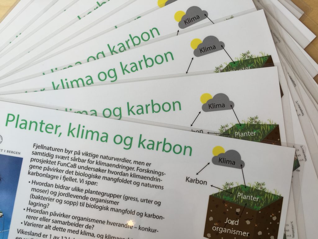
We have started a new project called FunCaB which tries to disentangle the roles of different plant functional groups, such as grasses, herbs and mosses. For this, we set up sites in boreal and alpine grasslands where we are removing these functional groups. And this means sitting for hours in front of a plot and cutting grasses or picking bryophytes. We will then measure how species composition is affected and how carbon dynamics changes when removing certain functional groups.

This one day in the field was nice, but also thought me how tough this task is. It is tedious work and we need a lot of helping hands to fulfill the task. So, thanks a lot to Linn and the students helping to get this work done!

FunCaBplots

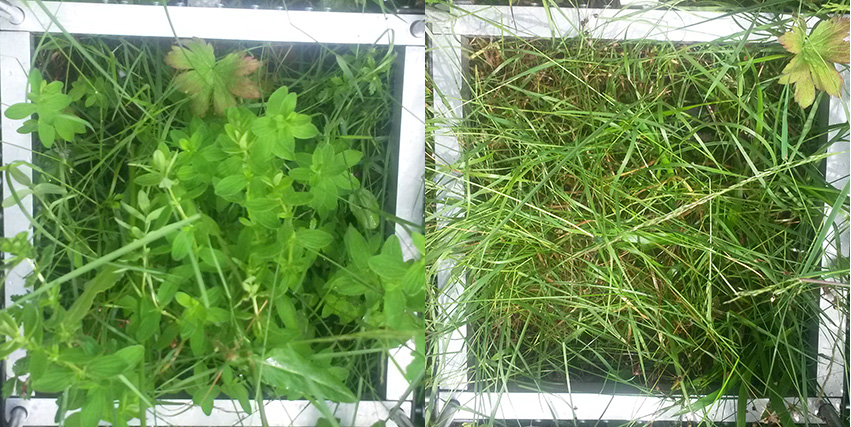
The pictures show a plot before and after removing the herbs.

Save and load

Save and load a R object can be very useful. A common way to store your results in R is to create a txt, csv or xls file. The advantage is that you can open the tables with many programs on your computer. But as soon as you want to do something with it in R it becomes complicated. You need to import the csv file back into R. You need to define header, how the data is separated. And you can never be sure if a factor is still a factor or a date is still a date. Usually, there are some complications that need to be fixed.

An easier solution is to use the function “save” to store your R object. The advantage here is that all the properties of the object are retained. For example a data frame will be a data frame again, a list will be opened as a list.

Let’s create a data set.

# create a data set
petal.length <- rnorm(100, mean = 2.5, sd = 1)
petal.width <- rnorm(100, mean = 1.75, sd = 1)
species <- rep(letters[1:10], each = 10)
floral.traits <- data.frame(species, petal.length, petal.width)

# here we have specis as a factor and two numeric variables
str(floral.traits)
## 'data.frame':    100 obs. of  3 variables:
##  $ species     : Factor w/ 10 levels "a","b","c","d",..: 1 1 1 1 1 1 1 1 1 1 ...
##  $ petal.length: num  2.4 3.08 3.5 2.75 2.92 ...
##  $ petal.width : num  1.525 2.138 2.397 2.148 0.838 ...

Now let us do somthing with this data, for example calculate the mean petal length and petal width for each species.

# calculate mean petal length and withd for each species
mean.pl <- tapply(floral.traits$petal.length, floral.traits$species, mean)
mean.pw <- tapply(floral.traits$petal.width, floral.traits$species, mean)
# transpose the data to make the table easier to handle and combine the means to one data set.
means <- data.frame(t(rbind(mean.pl, mean.pw)))
means$species <- factor(rownames(means)) # add speceis column

We have calculated the mean petal length and width for each species. And now we want to store this result. Maybe we want to use this result later to plot or calculate something. But let’s save it for now with the function “save”.
The first argument is the name of the object you want to save or a list of objects. File is the name of the file with RData at the end. There are more options, but you will mostly use the two first arguments.

# save the R object
save(means, file = "MeanPetalLengthAndWidth.RData")
# let's remove the data set to make sure this is working.
rm(means)

Your R object is now stored in the working directory you are using. We also removed the object from the environment to make sure the object is saved and we can reload it again.

Now we want to load the object back again to our environment to use it further. For this we use the “load” function. The first argument here is the file name. With envir you define where the data should be loaded to. And with verbose you can decide if you want the item name to be printed or not. This can be useful if you have forgotten what it was called.

# load the R object
load("MeanPetalLengthAndWidth.RData", verbose = TRUE)
## Loading objects:
##   means
# check the properties of the object.
str(means)
## 'data.frame':    10 obs. of  3 variables:
##  $ mean.pl: num  2.56 2.34 2.68 2.32 3.23 ...
##  $ mean.pw: num  1.82 1.76 1.75 1.74 2.34 ...
##  $ species: Factor w/ 10 levels "a","b","c","d",..: 1 2 3 4 5 6 7 8 9 10

Now you can check if the object has reapeard in the environment. And then you can . Have fun saving and loading!

# Barplot of petal length
barplot(means$mean.pl, names.arg = means$species, ylab = "Petal length", xlab = "Species")

plot of chunk unnamed-chunk-5

Plant Functional Trait Course in China

The 2016 International Plant Functional Traits Course will offer a hands-on, field-based exploration of plant functional traits, along with experience in the usage of plant traits data in climate-change research and ecosystem ecology. Trait-based ecology offers an important set of methods and new approaches that enables a more powerful approach to predict how climate and biotic interactions shape the diversity of communities and functioning of ecosystems. This course will provide students with the essential background and skills needed for trait-based ecology.

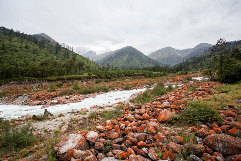
Red stones

Blogging directly from R using RWordPress

My last blog post was published using RMarkdown. It took me a while to intall all the packages needed but the publishing was very easy.In fact, it is 2 lines of code. But let’s start with the hard part getting all the packages installed and running.

The RWordPress package is currently on github (February 2016). It can be installed directly from there, but for that the devtools package is needed. To connect to WordPress we need the XMLRPC package. And you need of course the RWordPress package and the knitr package to make the blog post.

Let’s install the packages.

install.packages("devtools")
library(devtools)

install_github("duncantl/XMLRPC")
install_github("duncantl/RWordPress")
install.packages("knitr")

library(XMLRPC)
library(RWordPress)
library(knitr)

Once your blog post is writen you can check how it looks. For this you press the “Knit HTML” button on top (in R Studio). If everything looks fine, you are ready to publish. With options you define your username, password and url with “xmlrcp.php” at the end.

In “knit2wp” you define the filename of the Rmd document and the title of the blog post. You can publish directly, but by setting publish = FALSE you can make a draft and publish it later. With action you can create a new or edit an existing post.

options(WordPressLogin = c(user = 'Password'), WordPressURL = 'https://audhalbritter.com/xmlrpc.php')
knit2wp('RWordPress.Rmd', title = 'Blogging directly from R using RWordPress', publish = FALSE) 

You can find more information here and here:
http://yihui.name/knitr/demo/wordpress/
http://3.14a.ch/archives/2015/03/08/how-to-publish-with-r-markdown-in-wordpress/

Have fun bloggin!